R Workflow
Nowadays, there seems to be an R package for anything and everything. While this makes starting a project in R seem quick and easy, there are considerations to take into account that will make your life easier in the long run.
Working with OnDemand, not against
Having multiple R OnDemand sessions running that utilise the same library may
cause issues. It is best to ensure that all idle sessions have been exited
properly and the jobs have been deleted from the Active Jobs page which can
be found under the Jobs tab in OnDemand. If multiple sessions are needed, try
to ensure that they don't interfere with each other.
Understanding your environment
When beginning a project, keep the scope in mind and build your environment accordingly. Trying to build a universal environment that holds all the packages you could ever need will lead to incompatibilities at some point in the future.
Getting comfortable clearing your environment (not just sweeping your session variables) is essential to having a functional library. This is done with the following command:
rm -rf ~/R/x86_64-pc-linux-gnu-library
Note this removes all R libraries. Specific libraries can be removed by following this method, documented in a previous blog post.
Simplify the installation
Once you've cleared your environment, creating an installation script for a given environment will reduce your installation time, and ensure a clean slate.
Below demonstrates installing an R environment within an Apocrita job script, using 4 cores:
#!/bin/bash
#$ -cwd
#$ -pe smp 4
#$ -l h_rt=1:0:0
#$ -l h_vmem=1G
#$ -j y

mkdir -p /data/home/$USER/R/x86_64-pc-linux-gnu-library/4.2

module load R

Rscript 01_install_env.R
The mkdir command is run only once after your environment has been cleared.
Also, note that the above mkdir command is creating a R 4.2 environment,
which should match the working R version.
Below shows the contents of the 01_install_env.R file:
install.packages("dplyr")
install.packages("DESeq2")
install.packages("ggplot2")
install.packages("pheatmap")
Defaults for quick and consistent installation have already been specified for
you, such as setting the mirror to
cloud and using
multiple cores.
Save to file frequently
As natural breakpoints in your project arise, take the opportunity to save the relevant datasets and/or plots to file.
Reading from file is much more effective and reproducible than repeating a series of commands time and time again.
If you are concerned about space, you can write and read to a gzipped file
using write.csv() and read.table() respectively.
This will result in more intermediary files being created so keeping your raw
and processed data directories organised is essential.
Modularise your scripts
Instead of creating a script that is a collection of processes, we recommend creating shorter scripts, each one with a specific purpose. By starting each script name with a number, it is easier to keep track of the workflow. For example, a possible differential expression workflow:
01_install_env.R
02_preprocess_data.R
03_DE_analysis.R
04a_plot_volcano.R
04b_plot_heatmaps.R
From there, only load packages that are relevant to that script. In this
example, DESeq2 is only loaded in script #3 and ggplot2 (or likewise) is
only loaded in scripts #4a and #4b.
Start with small data
Build your scripts in OnDemand or an interactive session with only a portion of the data you will ultimately be analysing. This way, you can test and tweak functions and visualisations.
Before moving onto the entire dataset, it is helpful to understand all the data
types using Exploratory Data Analysis (EDA) techniques (table() etc.) to
predict possible errors.
Example full workflow
Once the scripts are finalised and the data are properly documented with data dictionaries or similar, running a qsub job script on the entirety of the data will be the most reproducible way to finalise the project. I would always recommend doing this before moving onto another script or project. To help with debugging, ensure that logs are being written to file.
Each script will be writing to file and the next will be reading from file. All that is needed to run the entire project would be:
#!/bin/bash
#$ -cwd
#$ -pe smp 1
#$ -l h_rt=1:0:0
#$ -l h_vmem=1G
#$ -j y

module load R

Rscript 02_preprocess_data.R
Rscript 03_DE_analysis.R
Rscript 04a_plot_volcano.R
Rscript 04b_plot_heatmaps.R
Note that one core is being requested for the full analysis, as these scripts only have the capability to run using one core.
Exit intentionally
While idle RStudio sessions will no longer timeout, it is best to quit
each session instead of letting them run out. To do this, save your work,
remove no longer needed session variables, select "Quit Session...", and close
the browser tab. This can be done even if your code is still running but you
don't plan on interacting with it. When you are ready to work on it and
resources still remain on your job, you can get back to your RStudio session
from your My Interactive Sessions tab.
Extra: Global Options
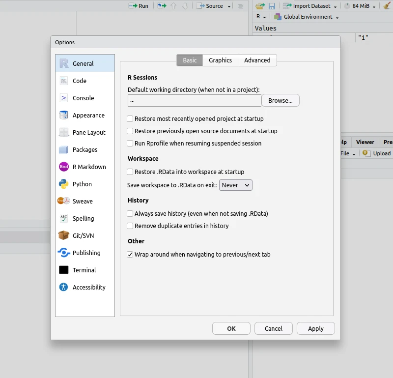
With the recommendations listed above, resuming work in R (interactively or OnDemand) should be painless. To avoid any unpredictable hiccups, it is best to keep your Global Options as shown below:
Note that any "Restore" option should be unchecked. This ensures RStudio does not attempt to load previous data or session configurations (which has been known to cause problems).
However, if you are more comfortable maintaining old sessions (and settings), be sure to clear any extraneous variables before ending each session. You will not be able to enter a new session if the stored variables exceed the amount of resources requested.
Title image: Cris DiNoto on unsplash


